SVM 多项式核¶

张**

In [1]:

%pylab inline

import numpy as np
import skimage.io as SKimg
import matplotlib.pyplot as plt
from sklearn.cluster import KMeans
from sklearn import mixture
from sklearn import metrics
import matplotlib.pyplot as plt
from mpl_toolkits import mplot3d
from skimage import io,data

Populating the interactive namespace from numpy and matplotlib

In [2]:

def MyStand(img,cof):
    roi1=copy(img)
    roi1[roi1!=255]=0
    roi1[roi1==255]=1
# # roi1[roi1==255]=1
    roi1=roi1*cof
    return roi1

In [3]:

from sklearn.decomposition import PCA
img=SKimg.imread("G:\\test\\Hyperspectral_Project\\dc.tif")
print(img.shape)
# img = np.transpose(img,(1,2,0))#(1280, 307,191)
# print(img.shape)

# img=[:,0:500,100:200]
img=img[:,0:500,:]#（191，500, 100）
print(img.shape)

X =img.reshape(191,153500)
# X2 =X.reshape(191,1280,307)

# # plt.imshow(X2[50,:,:])
# plt.imshow(img[50,:,:])

# X_pca=X[(59,26,16),:]
pca = PCA(n_components=3)
pca.fit(X)
print(pca.explained_variance_ratio_)

X_pca=pca.components_

print(X_pca.shape)

(191L, 1280L, 307L)
(191L, 500L, 307L)
[ 0.86881155  0.11072629  0.01735181]
(3L, 153500L)

In [4]:

# import Image
from PIL import Image
roof = imread('G:\\test\\Hyperspectral_Project\\1roof.bmp')
roi1=MyStand(roof,1)


street = imread('G:\\test\\Hyperspectral_Project\\2street.tif')
roi2=MyStand(street,2)


path = imread('G:\\test\\Hyperspectral_Project\\3path.tif')
roi3=MyStand(path,3)

grass = imread('G:\\test\\Hyperspectral_Project\\4grass.tif')
roi4=MyStand(grass,4)

street = imread('G:\\test\\Hyperspectral_Project\\5tree.tif')
roi5=MyStand(street,5)

street = imread('G:\\test\\Hyperspectral_Project\\6water.tif')
roi6=MyStand(street,6)

street = imread('G:\\test\\Hyperspectral_Project\\7shadow.tif')
roi7=MyStand(street,7)

# street = imread('G:\\test\\Hyperspectral_Project\\8other.tif')
# roi8=MyStand(street,0)

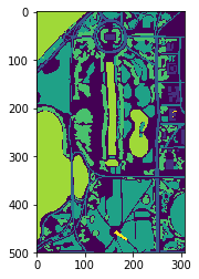
roi=roi1+roi2+roi3+roi4+roi5+roi6+roi7
roi_=roi[0:500,:]

plt.imshow(roi_)#[0:500,100:200])
# plt.savefig('G:\\roi.tif')
# roi_img=Image.fromarray(roi)
# roi_img.save('G:\\roi2.tif')

Out[4]:

<matplotlib.image.AxesImage at 0xe504588>

../../_images/StudentReports_2018Student_SVMPolyKernel_5_1.png

In [6]:

# X_pca=X_pca[:,0:500,100:200]
# plt.imshow(X_pca[1,0:500,100:200])
print(roi_.shape)
print(X_pca.shape)

(500L, 307L)
(3L, 153500L)

In [9]:

X_pn = np.transpose(X_pca,(1,0))
X=X_pn
Y=roi_new.flatten();
print(X_pn.shape)
print(roi_new.shape)

(153500L, 3L)
(153500L,)

In [10]:

from sklearn.model_selection import train_test_split
from sklearn.linear_model import LogisticRegression
from sklearn.metrics import accuracy_score
from ipywidgets import interact,interact_manual

In [11]:

X_train, X_test, y_train, y_test = train_test_split(
        X,
        Y,
        train_size=0.75)

D:\Anaconda2\lib\site-packages\sklearn\model_selection\_split.py:2026: FutureWarning: From version 0.21, test_size will always complement train_size unless both are specified.
  FutureWarning)

In [12]:

print(X_test.shape)

(38375L, 3L)

In [13]:

#训练模型
from sklearn.svm import SVC

clf = SVC(C=1E2,kernel='rbf',gamma='auto').fit(X_train, y_train)

In [14]:

clf.score(X,Y)

Out[14]:

0.62461889250814329

In [15]:

clf.score(X_test, y_test)

Out[15]:

0.62538110749185671

In [19]:

y_model = clf.predict(X_test)
accuracy_score(y_test, y_model)

Out[19]:

0.62538110749185671

In [20]:

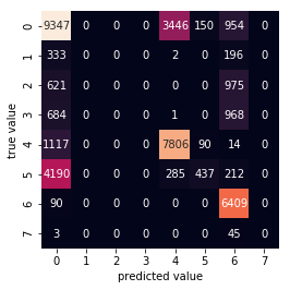
import seaborn as sns
from sklearn.metrics import confusion_matrix

mat = confusion_matrix(y_test,y_model)

sns.heatmap(mat, square=True, annot=True,fmt='d', cbar=False)
plt.xlabel('predicted value')
plt.ylabel('true value');

../../_images/StudentReports_2018Student_SVMPolyKernel_15_0.png